Erasure Coding Overhead Analysis
Terms related to simplyblock
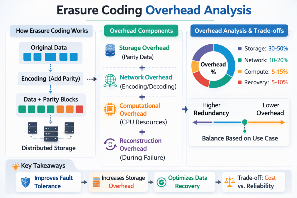
Erasure Coding Overhead Analysis shows what erasure coding really costs in a storage stack, beyond the raw capacity math. Teams track three types of overhead: extra capacity for parity, extra CPU for encode and rebuild, and extra latency from added work on the I/O path. In Software-defined Block Storage, those trade-offs decide whether you save money per usable terabyte or pay for it in tail latency.
Capacity overhead is easy to explain. A k+m scheme stores k data chunks plus m parity chunks, so raw capacity grows by (k+m)/k. Performance overhead takes more work. Writes trigger parity math. Reads may trigger decode work in degraded mode. Rebuilds can compete with application traffic for CPU cycles, cache, memory bandwidth, and network.
A useful analysis also separates “healthy” behavior from “failure” behavior. Many platforms look fast when the cluster stays healthy. Real systems must continue to run during maintenance, node loss, and rolling upgrades, so overhead must account for rebuild windows and degraded reads.
Cutting erasure-coding overhead with SPDK-based I/O
You reduce overhead when you cut CPU waste per I/O. User-space, zero-copy I/O paths help by avoiding extra copies and context switches. SPDK-style designs also keep work on dedicated cores, which helps steady latency under load.
Architecture choices matter as much as code choices. Hyper-converged storage often keeps traffic local, which lowers network fan-out and reduces the chance that east–west congestion inflates p99. Disaggregated storage can scale and isolate better, but it raises the bar on fabric design, QoS, and rebuild control. Most enterprises end up running a mix of both across environments, especially on bare-metal clusters where they want a SAN alternative without specialized arrays.
🚀 Reduce Erasure Coding CPU and Rebuild Cost on NVMe/TCP
Use simplyblock’s advanced erasure coding to keep Kubernetes Storage fast while you protect data efficiently.
👉 Use simplyblock for Advanced Erasure Coding →
Erasure Coding Overhead Analysis in Kubernetes Storage
Kubernetes Storage adds platform overhead that classic SAN teams do not model. The scheduler moves pods. Nodes come and go. CSI actions add, attach, and mount work. Multi-tenant clusters create noisy-neighbor risk, so one rebuild can hurt an unrelated workload unless you enforce strong isolation.
A solid Erasure Coding Overhead Analysis starts with placement rules. Match your erasure coding groups to real failure domains, such as node, rack, or availability zone. Then confirm that the system keeps fragments spread correctly during rebalancing. If fragments bunch up, you lose protection and waste rebuild effort.
Kubernetes also changes how you plan headroom. Build for peak plus recovery, not just peak. When you size only for steady state, rebuilds push nodes into saturation, and tail latency spikes.
Erasure Coding Overhead Analysis and NVMe/TCP
NVMe/TCP makes NVMe-oF practical on standard Ethernet, which helps teams standardize the fabric. It also puts real work on host CPUs compared to RDMA, so CPU headroom becomes part of the overhead budget.
In NVMe/TCP environments, erasure coding can stress three hotspots at once: parity math, packet processing, and memory bandwidth. When those hotspots collide, latency climbs first, then throughput falls. You can limit the risk by keeping the data path lean, by pinning critical threads, and by enforcing QoS so rebuild work cannot starve foreground I/O.
Teams that run mixed fabrics often start with NVMe/TCP for broad compatibility, then add NVMe/RDMA where certain workloads demand tighter tail latency. Either way, the analysis must cover transport costs, not just capacity ratios.
Measuring and Benchmarking Erasure Coding Overhead Analysis Performance
Benchmarking should mirror how the workload behaves, not how a lab demo behaves. Start with a profile that matches block size, read/write mix, and queue depth. Next, run the same profile during degraded mode, and again during rebuild. Compare p50, p95, and p99 latency, plus CPU per node, network bandwidth, and rebuild completion time.
Avoid “one number” reporting. Average latency hides pain. Tail latency reveals it.
Use this single checklist to keep results comparable:
- Capture p50, p95, and p99 latency for reads and writes, plus IOPS, throughput, and CPU per node.
- Run healthy, degraded, and rebuild tests with the same workload profile and the same dataset size.
- Test with a rebuild rate cap, then test without a cap, and record the change in p99 latency.
- Repeat at low and high utilization, because overhead grows fast near saturation.
Ways to speed up parity math and rebuilds
You improve results when you control contention first. Reserve CPU for foreground I/O. Put hard limits on rebuild bandwidth during peak hours. Let rebuild run faster during off-peak windows. Those controls often deliver bigger gains than switching from one k+m layout to another.
Stripe size also changes behavior. Smaller stripes can rebuild faster and reduce exposure time, but they can raise write overhead. Larger stripes improve capacity efficiency and can reduce parity overhead per usable terabyte, but they increase fan-out and can raise network pressure.
Finally, treat multi-tenancy as a design goal, not an afterthought. Strong isolation and QoS prevent one tenant’s burst or rebuild from pushing other tenants past their SLO.
Usable Capacity Impact Across Replication and Erasure Coding
The table below shows raw capacity overhead for common protection schemes. Use it as a starting point, then validate CPU cost and tail latency on your own Kubernetes Storage and NVMe/TCP setup.
| Protection scheme | Example layout | Raw capacity multiplier | Extra raw capacity vs usable | Practical impact |
|---|---|---|---|---|
| Replication | 2× copy | 2.00× | +100% | Simple recovery, higher capacity cost |
| Erasure coding | 4+2 | 1.50× | +50% | Faster rebuild, higher write cost |
| Erasure coding | 8+2 | 1.25× | +25% | Better capacity use, higher fan-out |
| Erasure coding | 16+4 | 1.25× | +25% | More fragments per I/O, needs strong QoS |
Simplyblock™ controls for erasure-coded pools
Simplyblock targets high performance on NVMe and NVMe/TCP, while keeping erasure-coded pools efficient in Kubernetes Storage. Simplyblock uses an SPDK-based, user-space approach to reduce CPU overhead in the hot path, which helps protect tail latency when the cluster runs near peak.
Operators also need control, not just speed. Simplyblock focuses on multi-tenancy and QoS, so platform teams can isolate workloads, reserve performance for critical volumes, and limit the blast radius of rebuilds. Those controls matter most during node loss, rolling maintenance, and noisy-neighbor events.
Roadmap for lower overhead at scale
Teams will push more work into offload paths. DPUs and IPUs can reduce host CPU load for packet handling and parts of the storage stack, which helps NVMe/TCP environments stay stable under pressure. Platforms will also tighten placement automation, so they keep shards spread across the right failure domains during growth and rebalance.
Rebuild logic will keep improving, too. Systems that prioritize hot data first can reduce user-facing latency swings while still completing recovery. Better observability will close the loop by linking SLO targets to rebuild rate, QoS limits, and placement choices.
Related Terms
Teams often review these glossary pages alongside Erasure Coding Overhead Analysis.
Hybrid Erasure Coding
CRUSH Maps
Zero-copy I/O
IO Path Optimization
Questions and Answers
Erasure coding overhead is the ratio of raw capacity consumed to usable capacity, typically (k+m)/k. For example, 8+2 uses 1.25x raw (25% overhead), while 4+2 uses 1.5x raw (50% overhead). This is the baseline “space tax” before considering metadata, padding, and rebuild reserve. The core concept is covered in erasure coding.
Small random writes often trigger read-modify-write at the stripe level: the system must read old data/parity, recompute parity, then write updated shards. That creates extra backend I/O beyond what the app issued and can inflate tail latency. The penalty depends on stripe width, write size alignment, and caching. This is closely related to write amplification effects in distributed systems.
Parity encoding adds CPU cost on writes, while decoding adds CPU cost on degraded reads and rebuilds. The overhead scales with throughput, code type, and SIMD acceleration; it can become the bottleneck before disks do, especially on fast NVMe + high-speed networks. If CPU saturates, queues build, and p99 latency rises even when the storage media is idle.
Erasure coding typically fans out a write across more peers (k+m shards) and may require cross-node reads for partial-stripe updates, increasing east-west traffic. Replication sends full copies but usually avoids parity reads on update. Under failure, erasure coding reconstructs from multiple nodes, which can spike network usage and amplify latency variability relative to replication.
A useful overhead analysis separates: space overhead ((k+m)/k), write I/O overhead (read-modify-write), CPU overhead (encode/decode), and network overhead (shard fanout + degraded reconstruction). Then add operational overhead: reserved headroom for rebuilding windows and performance impact during failure. Reporting all five avoids the common mistake of treating erasure coding as “only a capacity equation.”